Cell segmentation and image analysis with Cellpose, no code required

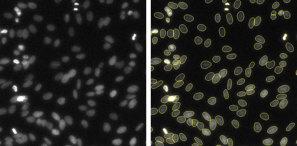
Finding and measuring cells in microscopy images should not require researchers to toil away troubleshooting environments. Yet for many scientists, running a state-of-the-art segmentation model still means installing packages, fixing version conflicts and editing scripts before a single cell is counted.
We built a free Google Colab notebook that removes all of that. It runs Cellpose, the widely used deep learning segmentation tool, on Google's cloud GPUs. Every step is a single button. The code is still there, but it is folded away behind simple forms, so you never have to read it, edit it or even see it.
You upload your images, click ▶ five times, and download a zip folder of masks, outlines and per-cell measurements. This post walks through each click. Get the free notebook.
Why Google Colab instead of your own computer
Cellpose runs on your own computer too, and most modern laptops even have a GPU in them. But that GPU was built to render your screen, not to run a deep learning model on a folder of images for minutes or hours at a time. Colab hands you a cloud computer built for exactly that, for free:
- Speed. Cellpose-SAM segments a 512 × 512 image and finds cells in under a second of inference time on Colab's cloud GPU. Your own computer's CPU would take several times longer per image, and that gap widens on larger or multi-channel images.
- Batch scale. The notebook loops over every file you upload, so the same five clicks handle 5 images or 500. Queue up a whole plate's worth of fields of view, click Segment once, and walk away. On your own computer's CPU that could mean hours, and it ties the machine up the whole time. On Colab's cloud GPU it is minutes.
- No setup, no conflicts. There is no CUDA driver to install, no GPU to buy, and no clash with whatever else is on your computer. Colab gives you a clean environment every session.
- It costs nothing to start. Colab's free tier includes cloud GPU time, with usage limits that reset regularly. Heavier use can move to Colab Pro or a paid cloud GPU, still far cheaper than a dedicated workstation.
What you need
- A Google account. Colab is free and runs in your browser. Nothing is installed on your computer.
- Your images. TIFF, PNG, JPG or BMP, uploaded one by one or as a single zip folder. Multi-channel images work, and 3D z-stacks are max-projected automatically.
- About three minutes. Most of that is a one-off install. Segmentation itself takes seconds per image on the free GPU.
No Python knowledge is needed at any point.
Step by step
This walkthrough uses a single 512 × 512 fluorescence image of nuclei from the 2018 Data Science Bowl dataset (BBBC038, CC0), on Colab's free T4 GPU.
1. Open the notebook in Colab
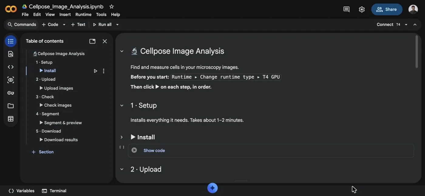
Click Get the free notebook and it opens straight in Google Colab, in your browser: no download and nothing to install. You will see five numbered steps, each with a single ▶ button, and no code on screen. Each step is a form with a title, a short description and, where needed, a dropdown.
2. Setup
Click ▶ on Install. If Colab warns that the notebook was not authored by Google, click Run anyway. The install takes about a minute and ends with a green card confirming the GPU is on.
3. Upload
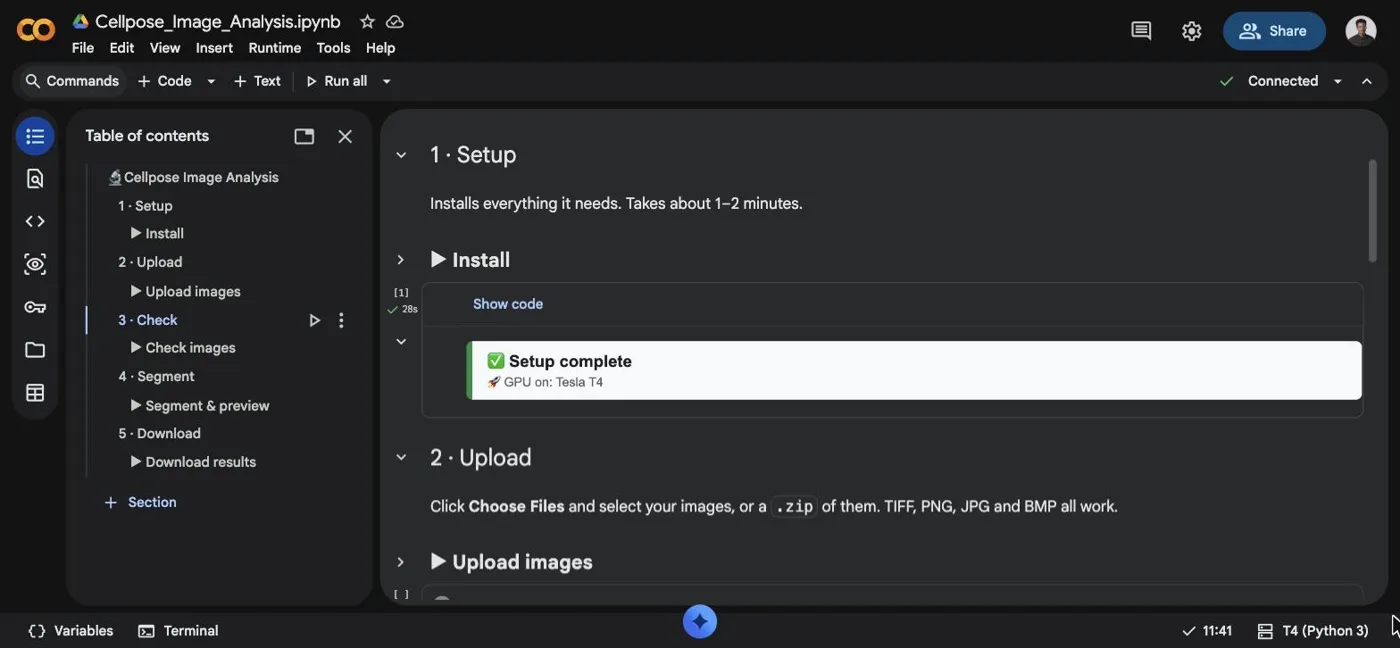
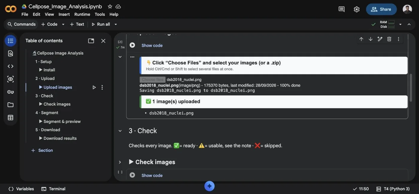
Click ▶ on Upload images, then Choose Files. Select one image, several, or upload them all together as a zip folder. A green card confirms how many arrived.
4. Check
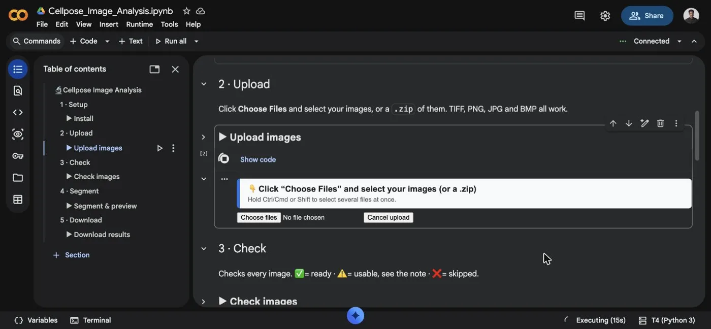
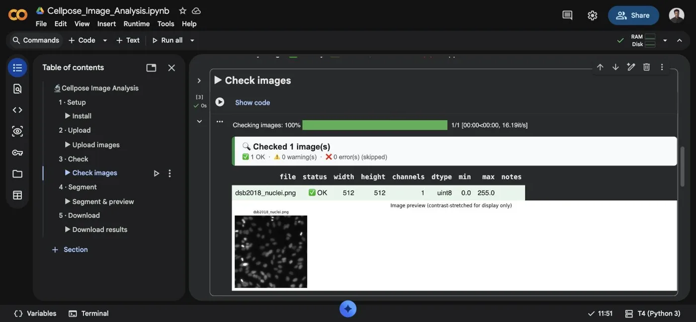
Click ▶ on Check images. Every file is checked before any analysis runs, so problems show up early rather than halfway through a batch. Each image gets a status (✅ ready, ⚠️ usable with a note, ❌ skipped) with its size, channels and bit depth, plus thumbnails of the first ten images, for a visual confirmation.
5. Segment
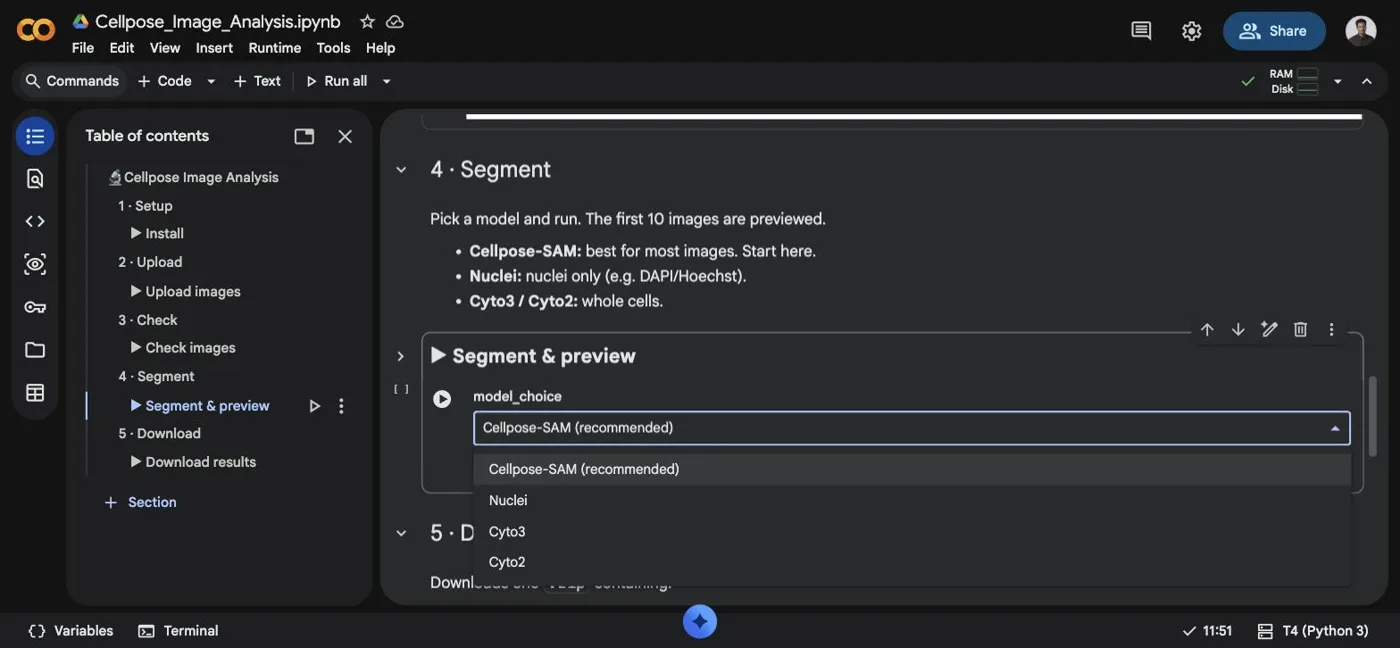
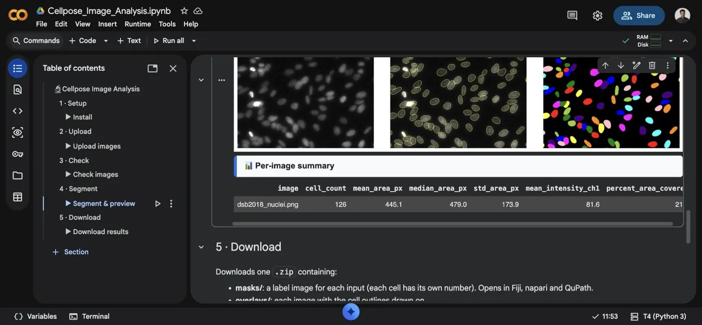
Pick a model from the dropdown and click ▶. Cellpose-SAM is selected by default and is the best starting point for most images. You get a side-by-side preview of the original, the detected outlines and the coloured masks, plus a summary table for each image.
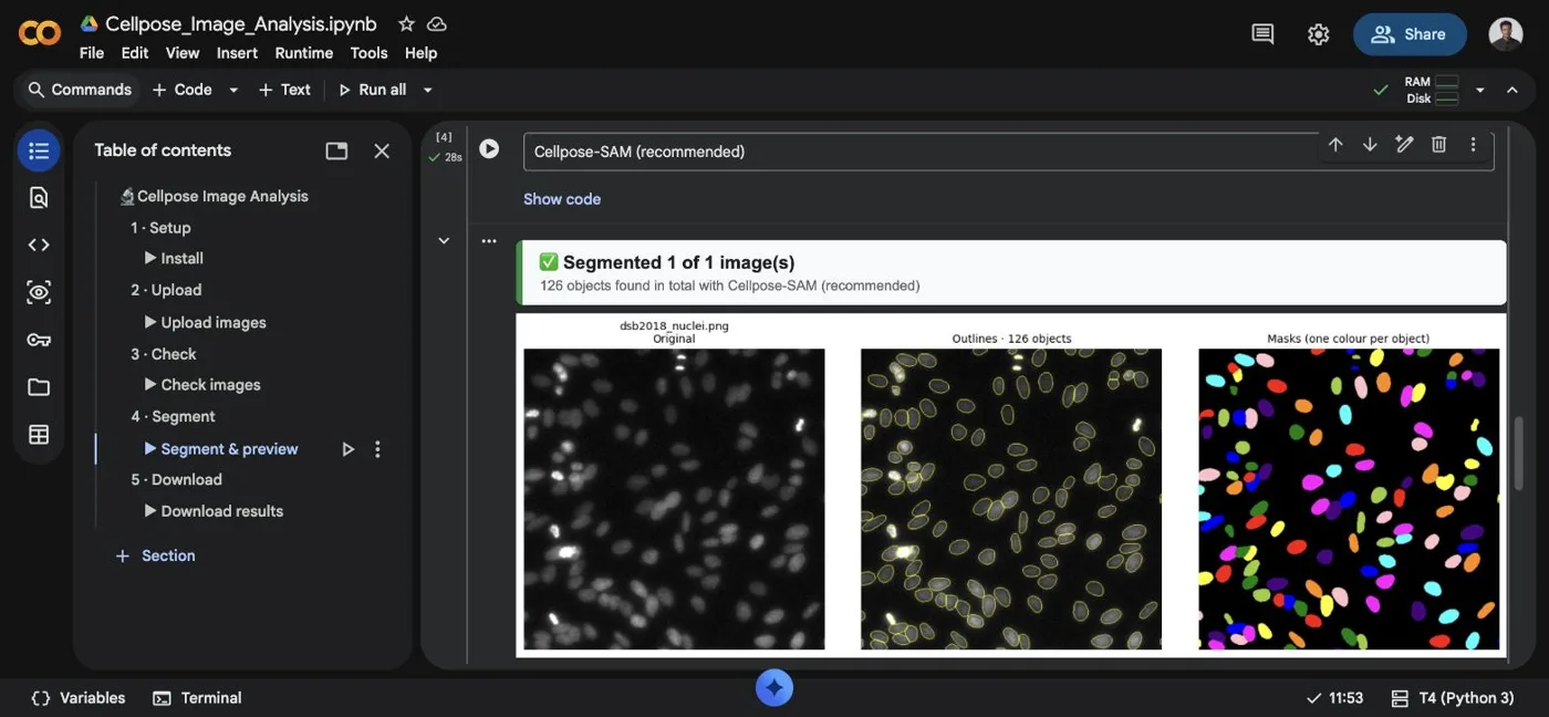
The summary table gives the cell count, mean and median area, and the percentage of the image covered.
6. Download
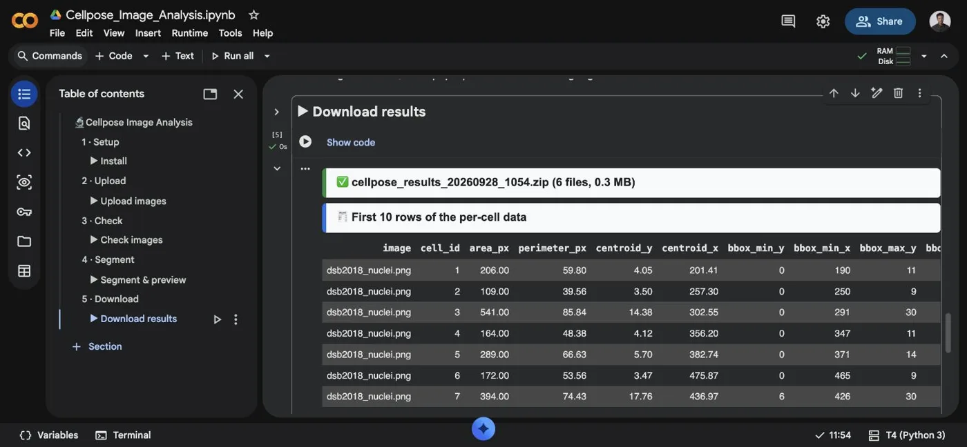
Click ▶ on Download results. A single zip folder (six files) downloads to your computer, and the first ten rows of per-cell data appear below so you can sanity-check them straight away. If nothing downloads, allow pop-ups for colab.research.google.com.
The code is there when you want it
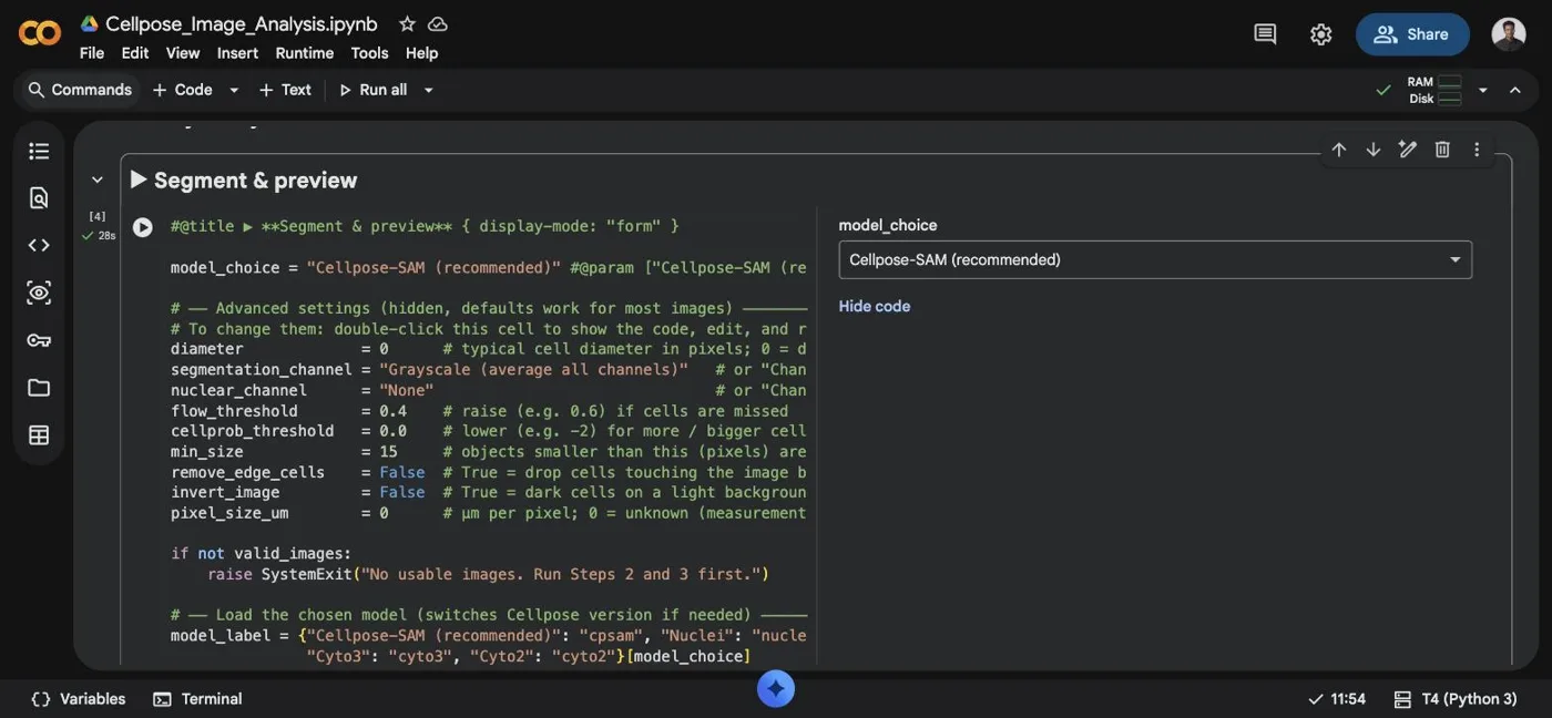
Nothing is locked away. Click Show code on any step and the full, commented code opens beside the form. Most users will never need it, but it means the analysis is transparent and auditable, and easy to adapt if your lab has a specific need.
What you get back
One timestamped zip folder, organised so each file is ready for the next tool in your workflow.
| File or folder | What it contains | Use it for |
|---|---|---|
| masks/ | A 16-bit label image per input, each cell with its own number | Further analysis in Fiji, napari or QuPath |
| overlays/ | Each image with yellow cell outlines drawn on | Quick visual QC, slides and figures |
| measurements/ | One CSV per image, one row per cell | Per-image analysis |
| all_cells_measurements.csv | Every cell from every image in one table | Statistics across conditions in Excel, Prism or R |
| summary_per_image.csv | Cell count, mean and median area, % area covered | Counting and confluence at a glance |
| analysis_settings.csv | Model, Cellpose version and every parameter used | Reproducibility and methods sections |
Each cell is measured for area, perimeter, centroid, bounding box, eccentricity, solidity, major and minor axis length, orientation and equivalent diameter. Mean, minimum, maximum and integrated intensity are reported for every channel in the original image, not only the one used for segmentation.
Tips and honest limitations
Picking a model. Cellpose-SAM is the default and the best starting point for almost any image: it generalises across cell types and stains without you having to set a cell diameter. Nuclei is trained specifically on nuclear stains such as DAPI or Hoechst, and finds nuclei more reliably when that is all you have. Cyto3, and the older Cyto2, are trained for whole-cell boundaries, cytoplasm included, so reach for one of them when you need the full cell outline rather than just the nucleus, for example brightfield or membrane-stained images. If cells are still missed or merged, try one of the others. The notebook swaps between Cellpose versions for you, which adds about 30 seconds.
When you need more control. The defaults suit most images, but a small set of
advanced settings sits in the Step 5 cell, each with a one-line comment. Click Show code on
that step to reveal them. The two worth knowing are pixel_size_um, which converts
measurements from pixels to µm, and invert_image, for dark cells on a light
background such as brightfield or H&E.
Things to be aware of:
- Download before you close the tab. Colab deletes everything when the session ends.
- Free GPUs are not guaranteed. Colab allocates them on availability and ends idle sessions. Without a GPU the notebook still works, just more slowly.
- Your images are processed on Google's servers. Check your institution's policy before uploading sensitive or unpublished data.
- It is 2D. Z-stacks are max-projected before segmentation, which suits counting and area but not true 3D morphology.
- The models are pretrained. They perform well on common cell types and stains, but unusual cell lines or imaging setups may need parameter tuning, or a model fine-tuned on your own data.
If your cells fall into that last category, CellOpsis adapts segmentation models to your own cell lines and imaging setup, in the browser, with no code.
Get the free notebook
Tell us a little about yourself and the link appears straight away.
Your notebook is ready.
Open it in Colab, then use File ▸ Save a copy in Drive to keep your own version.
Open the notebook in Colab →If you use Cellpose in your work, please cite Stringer et al., Nature Methods (2021), and Pachitariu et al. (2025) for Cellpose-SAM.